1. Introduction
When an agent gives a wrong answer, the common reaction is to change the model. A newer model, a bigger one, or the same one with more reasoning effort. It is one line of configuration and it feels safe.
We build an agent that finds the root cause of incidents in Kubernetes clusters. In a previous post we described how we replaced a team of agents with one agent loop and what it bought us. This post is about a harder question. When we change something, how do we know the result moved because of the change and not because agents are noisy? We ran the same build twice on 21 problems and got results that differed by up to 38%. A comparison of that size has to beat that first.
The previous post reported the gains we saw when we made that change. This post asks how much confidence those comparisons deserve. Confirming the change on 84 problems it was never tuned on made one concern smaller, tuning to the benchmark, without ruling it out. It did not show how consistently the gain repeats across independent runs. The 1.5x of our previous post is the result without the Kubernetes tools, and on the 84 problems never used for tuning it is the 1.52x of Table 1. That is why the result of the previous post appears here as the strongest candidate and not as a finding.
We measured our changes in 61 runs and about 5,900 judged attempts. Table 1 has the result. To read it we did not need anything new, only basic statistics applied with some care.
The benchmark
The benchmark is SREGym. It deploys an application on Kubernetes, injects a fault and asks the agent for the root cause. An LLM judge gives each answer a score between 0 and 1, and an answer passes at 0.70. A run uses either the 21 problems of the lite set or about 105 problems of the full set, with 3 attempts on each problem.
The benchmark is only the instrument. The same methods apply to a replay of old incidents, to a judge or to a production signal.
2. Models versus the system
Table 1 compares each change with the version before it. Each row pairs two runs on the same problems and reports one ratio for the whole set. New over old is how often the new version passed over how often the old one did, so 1.00x means no change. The 95% interval shows how far that ratio moves when the mix of problems changes within those two runs. It does not include a shift that moves a whole run, so we also compare each ratio with how far two runs of the same build move apart on their own, which section 3 measures. On 21 problems that is 0.73x to 1.38x, and on about 100 problems we have no such range yet. The verdict follows from that. A ratio inside the range is not enough on its own, so the verdict is cannot tell. A ratio outside it is worth repeating, so the verdict is rerun candidate. A second pair only counts as confirmation when its rule was written before it runs, and no row is a finding yet.
| Change | Problems | New over old | 95% interval | Verdict |
|---|---|---|---|---|
| Sonnet 5.5 at high effort, against Sonnet 4.6 | 21 | 1.10x | 0.93x to 1.32x | cannot tell |
| Haiku 5.5, against Sonnet 5.5 | 102 | 0.93x | 0.87x to 0.996x | cannot tell |
| Sonnet 5.5 at low effort, against Sonnet 4.5 | 21 | 1.11x | 0.61x to 2.33x | cannot tell |
| Sonnet 5.5 at medium effort, against Sonnet 4.5 | 21 | 1.39x | 0.74x to 2.80x | cannot tell |
| Sonnet 5.5 at high effort, against Sonnet 4.5 | 21 | 1.67x | 1.05x to 3.14x | rerun candidate |
| Bundled system change, including one agent loop instead of a team, with Kubernetes tools | 84 | 1.25x | 1.15x to 1.39x | rerun candidate |
| Bundled system change, including one agent loop instead of a team, without Kubernetes tools | 84 | 1.52x | 1.31x to 1.82x | rerun candidate |
Table 1. Each side of a comparison is one run. Intervals come from resampling problems and do not include whole run shifts. The 21 problem rows are read against the same build range of section 3. The 84 problem rows have no such range yet, so they stay candidates until an independent repeat.
Only the Haiku change ran on about 100 problems. Its run differs from the Sonnet 5.5 run by one commit that lets the model accept its settings, and three of its problems did not deploy. It passed 0.93x as often, and counting the three missing problems in its favour moves the interval up to 1.01x. That drop is real in this pair, but one pair cannot tell how much of it comes from the model. The one near repeat at this size moved 0.97x, and one pair cannot show how far a whole run shifts, so we can neither call 0.93x a loss nor rule one out.
The Sonnet 5.5 changes ran on 21 problems, which is too few to size an effect. Against Sonnet 4.6, the model we were running at the time, the gain was 1.10x and inside the noise. A second judge then saw half the score gain against Sonnet 4.6, small enough to be noise. Against Sonnet 4.5, one generation further back, the gain looks larger. The high effort estimate is above the noise range, while its interval still overlaps that range. The medium effort estimate is on the edge.
The system change of our previous post is the strongest candidate. It bundled one agent loop in place of a team with an evidence ledger, a namespace scan and report checks. With the same model and the Kubernetes tools, the tools that let the agent query the cluster, it was better on 27 of the 84 problems we never tuned on and worse on 3. The two arms with the tools include a rerun of six problems. Without the tools the gain was larger.
Models still matter. We switched to Sonnet 5.5 because an attempt cost 0.53x what it did before, and because the live run on the same build showed no visible loss against Sonnet 4.6. That is a shipping decision, not a measured gain. A run of 21 problems cannot show that accuracy was preserved, so we wrote down before the switch which production signals would make us roll back. The checks below are what showed us how little any of the changes in Table 1 could be sized.
3. Run the same thing twice first
Before comparing two versions, we compared one version with itself. Figure 1 shows eight pairs of runs of the same build on the 21 problems. With nothing changed, the second run passed between 0.65x and 1.38x as often as the first. The totals also hide a second kind of noise. Two runs with the same pass rate can pass different problems. The number next to each bar is the agreement between the two runs on which problems passed, after discounting the easy problems both pass and the hard ones both fail (Cohen's kappa). 1 means they passed and failed the same problems. The pairs ranged from 0.34 to 0.73, so even a pair with a ratio near 1.0x did not pass the same problems. Higher is better, and ours is moderate, so a problem that flips between two runs is weak evidence on its own. Both numbers are noise we have to beat before any comparison, and the sections below are how we do it.
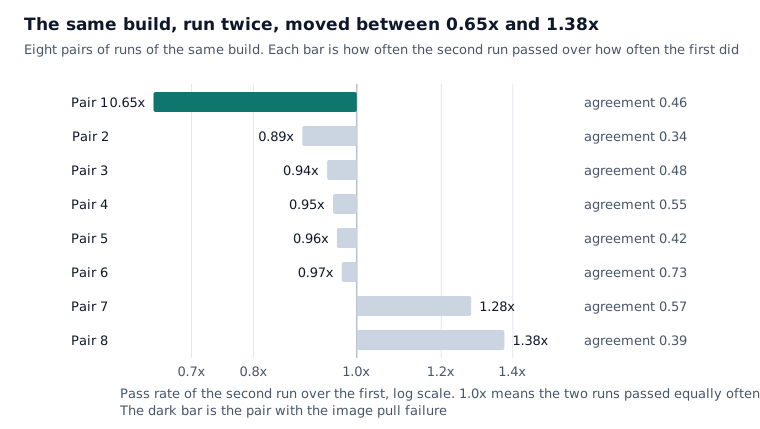
The worst pair, at 0.65x, would have been reported as a large regression if a model change had sat between the two runs. We went looking and found an image pull failure in the second run. Infrastructure noise looks exactly like a regression, so we keep that pair apart from the clean ones.
The seven clean pairs give the noise range behind the verdicts in Table 1. A new version can land on either side of the old one, so we take the range in both directions, 0.73x to 1.38x. Seven pairs is a small number, and the range is a guardrail, not a precise limit.
More problems shrink the noise in the average. On about 100 problems we have one near repeat pair, two commits apart, which gave 0.97x with an interval of 0.91x to 1.02x. That interval shows how far the mix of problems moves the ratio, which is the same kind of spread Table 1's own intervals show. One pair cannot show how far a whole run shifts at this size, so we have no noise range there yet.
4. Count problems, not attempts
A run of 21 problems with 3 attempts gives 63 verdicts, but not 63 independent observations. Attempts on the same problem tend to agree. Easy problems pass all three times and hard ones fail all three times. In our runs, all three attempts agreed on 62% of the problems. Once that is accounted for, 63 attempts carry about as much information as 33 independent ones.
So when we compare two versions, we count problems, not attempts, and compare each problem with itself across the two runs. That removes the difficulty of each problem from the comparison. It does not remove the shift between runs. Each arm of our comparisons was one run, so whatever moved that run as a whole is mixed with the change we were testing. That is why every ratio in Table 1 is read against the noise range of section 3.
5. Know what a run can detect
Before any run we ask what is the smallest gain it can reliably detect. We simulate it from our own runs. In our simulation, 21 problems with 3 attempts detect a gain of about 1.8x four times out of five. Every model change we measured on 21 problems had a smaller estimate than that, so those runs were never going to settle the question.
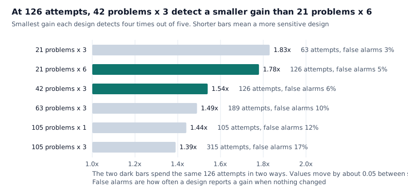
Because attempts on one problem agree with each other, it is better to add problems than repeats. With the same 126 attempts per arm, 42 problems with 3 attempts detect about 1.5x and 21 problems with 6 attempts about 1.8x.
More problems reduce the differences between individual problems. They cannot remove a shift shared by the entire run. A run wide shift moves every problem in the same direction, and the test can mistake that for a real improvement. In our simulation, false alarms rose from 3% on 21 problems to 17% on 105. A test that raises more false alarms also looks more sensitive, so the bars of Figure 2 do not rank the designs fairly. The shifts we reuse were measured on 21 problems and already contain the noise between problems, so the simulation counts that noise twice and the 17% is too high. Adding problems helps with the variation between problems. It does not replace repeating the comparison in independent runs, and that is the other reason every ratio in Table 1 is read against the same build range.
This check also stopped a planned parameter sweep before it ran. No sample we could afford would have detected the effect we expected.
6. Write the rule before the run
The rule we read Table 1 by was written while reporting, not before the runs. Of the comparisons in Table 1, only the Sonnet 5.5 migration had its criteria written down in advance. The others had no rule recorded, and that is what let us read them in whatever way the numbers suggested.
Now we write the rule before the run, and when we depart from it we record why. To merge a change, the problems it targets must clear a threshold written before the run, and the remaining problems must stay within an acceptable loss. In one case the target problems passed 5x as often and cleared the threshold we had written down. The change still failed the no harm check, so we did not merge it. The traces then showed that the harm came from an earlier change, merged without a before and after run.
Our first no harm check only asked whether the other problems got worse by more than chance would explain. A small run passes that easily, because a small run is bad at detecting anything. A no harm check should state how much loss we accept and require the interval to stay inside it. We now check the interval, but our merge rule does not yet state a margin.
7. Five checks before trusting an eval
Five more checks changed how we read Table 1. Each one is a step we now take before we trust a result.
Choose the metric before the run
The same runs told two different stories. Pass or fail showed no clear change for Sonnet 5.5 against Sonnet 4.6, while the judge's average score showed an improvement. Trying three effort settings also produced one apparent win on score, and it disappeared once we accounted for having tried three. Reasonable choices gave different headlines, so we now choose the metric and the test before the run.
A correlation is not an experiment. Attempts that ran a specific investigation step passed 3.3x as often as the others. So we prompted the agent to always run the step, in a paired experiment, and got the same number of passes in both arms.
Check the result a second way
The benchmark, the replay of old incidents and the LLM judge each measure something specific, so we check each one against a second one. A second judge from a different model family saw Sonnet 5.5's score gain at 0.036 instead of 0.069, small enough to be noise. The replay gives a changed agent the evidence of an old investigation, so it is much cheaper than a live run, but it cannot see an agent that collects less evidence, because the evidence is already there. The replay picked the cheapest effort setting of Sonnet 5.5. In the live runs that setting made a median of 33 tool calls per attempt where Sonnet 4.5 made 86. Fewer calls can mean a more efficient agent or one that skips evidence, and the replay cannot tell these apart, so we shipped the highest setting instead. The agent's own confidence is a weak signal too. It said it was at least 95% sure, and its error rate at that confidence was far above 5%.
Test on problems you never tuned on
A common loop is to look at the problems that failed, write a fix, run again and count how many pass now. Some pass anyway, because part of a failure is luck. After four fixes aimed at failing problems, the share of failing problems that then passed every attempt was 1.4x the share in a pair of runs with no fix at all, and the two were not distinguishable. That pair was not a matched control, because it used another build and model and a benchmark update sat between the before and after runs. So a targeted fix is now compared with a pair of runs of the same build on the same problems, run before the fix.
To avoid overfitting, we tune on one problem set and confirm once on a larger set. We tuned the system change on the 21 problems and confirmed it on the 84 problems of the full set that were never used for tuning. Table 2 shows both.
| System change | Tuned, 21 problems | Never tuned, 84 problems |
|---|---|---|
| With Kubernetes tools | 1.42x | 1.25x |
| Without Kubernetes tools | 1.35x | 1.52x |
Table 2. Pass rate of the new system over the old one, on the problems the change was tuned on and on the problems it never saw. Each ratio comes from one pair of runs, without an independent repeat.
The never tuned estimate had the same direction and a similar size. That is what we hoped to see, and it still does not rule out overfitting.
Check whether attempt order matters
Pooling attempts assumes that the three attempts on a problem are interchangeable. We tested this. Across the 48 runs on the 21 problems, attempt 3 passed 0.87x as often as attempt 1. Attempt 3 was below attempt 1 in 31 runs and above it in 12. A difference this uneven would happen by chance about once in 200 similar checks.
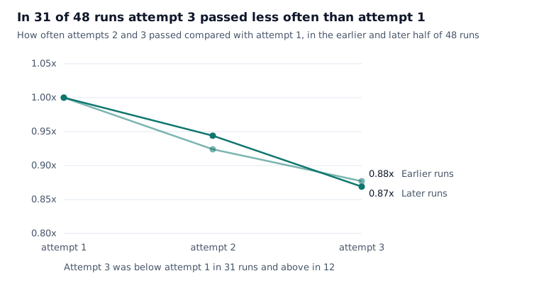
One explanation consistent with the traces is a bug in the benchmark harness. Attempts on a problem run one after the other in the same namespace, and in that reading the fault of one attempt is still visible to the next one. Order is also mixed with time within a run, so this is a hypothesis to test, not a finding. On the full set runs the result was inconclusive, with attempt 3 above attempt 1 in 6 of 9 runs. The scores never pointed at it. A simple test of an assumption did.
Let cost break the tie
Cost is measured much more precisely than accuracy. An attempt on Sonnet 5.5 cost 0.53x what it cost on Sonnet 4.6, and it was cheaper on every one of the 21 problems. On the same runs the pass rate did not move outside the noise. When accuracy cannot decide, cost often can.
Cost also finds bugs. Adding a judge step to the agent once raised the cost by 93% with no change in accuracy, because text that changed on every turn at the start of the prompt broke the prompt cache. Only the cost showed it.
8. What we change
A bigger or newer model is the easiest change to make and one of the hardest to measure. None of our model changes could be sized by our runs. The one on about 100 problems was a drop of 0.93x that one pair of runs cannot size, and a run of 21 problems could not size the others. Sonnet 5.5 shipped on lower cost and no visible loss. One result stood out. The bundled change to the system passed 1.25x as often with the Kubernetes tools and 1.52x without them, on 84 problems it had never been tuned on. It is the largest effect we measured and the only one measured off the tuning set, and the gain without the tools matters most because that is the posture production runs in. It is still one pair of runs, so it is a candidate and not a finding.
Three things change in how we evaluate. A candidate becomes a finding only when a second pair of runs repeats it under a rule written before the run. The thresholds of our decision rules come from pairs of runs of the same build, which means we run the same build twice. The attempt order effect gets tested as a harness bug. Two runs of the same build moved by up to 38%. Until we had measured that, every improvement we reported was a guess about the noise. Now the measurement comes first.